Deep Convolutional Generative Adversarial Network (DCGAN)

This is a beginner level tutorial for generating images of handwritten digits using a Deep Convolutional Generative Adversarial Network inspired by the TensorFlow tutorial on DCGAN.

What are GANs?

Generative Adversarial Neural Networks or simply GANs introduced by Goodfellow et al. is one of the most innovative ideas in modern-day machine learning. GANs are used extensively in the field of image and audio processing to generate high-quality synthetic data that can easily be passed off as real data.

A GAN is composed of two sub-models - the generator and the discriminator acting against one another. The generator can be considered as an artist who draws (generates) new images that look real, whereas the discriminator is a critic who learns to tell real images apart from fakes.

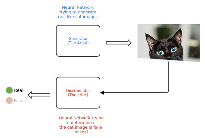
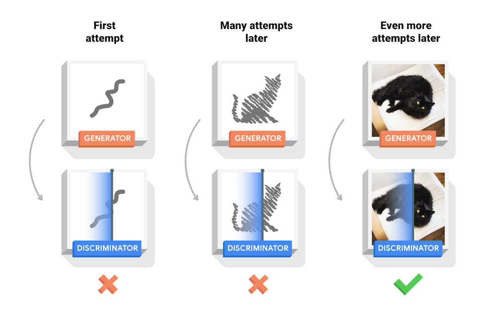
The GAN starts with a generator and discriminator which have very little or no idea about the underlying data. During training, the generator progressively becomes better at creating images that look real, while the discriminator becomes better at telling them apart. The process reaches equilibrium when the discriminator can no longer distinguish real images from fakes.

[source]

This tutorial demonstrates the process of training a DC-GAN on the MNIST dataset for handwritten digits. The following animation shows a series of images produced by the generator as it was trained for 25 epochs. The images begin as random noise, but over time, the images become increasingly similar to handwritten numbers.

Setup

We need to install some Julia packages before we start with our implementation of DCGAN.

using Pkg

# Activate a new project environment in the current directory
Pkg.activate(".")
# Add the required packages to the environment
Pkg.add(["Images", "Flux", "MLDatasets", "CUDA", "Parameters"])

Note: Depending on your internet speed, it may take a few minutes for the packages install.

After installing the libraries, load the required packages and functions:

using Base.Iterators: partition
using Printf
using Statistics
using Random
using Images
using Flux: params, DataLoader
using Flux.Optimise: update!
using Flux.Losses: logitbinarycrossentropy
using MLDatasets: MNIST
using CUDA

Now we set default values for the learning rates, batch size, epochs, the usage of a GPU (if available) and other hyperparameters for our model.

Base.@kwdef struct HyperParams
    batch_size::Int = 128
    latent_dim::Int = 100
    epochs::Int = 25
    verbose_freq::Int = 1000
    output_dim::Int = 5
    disc_lr::Float64 = 0.0002
    gen_lr::Float64 = 0.0002
    device::Function = gpu
end

Loading the data

As mentioned before, we will be using the MNIST dataset for handwritten digits. So we begin with a simple function for loading and pre-processing the MNIST images:

function load_MNIST_images(hparams)
    images = MNIST.traintensor(Float32)

    # Normalize the images to (-1, 1)
    normalized_images = @. 2f0 * images - 1f0
    image_tensor = reshape(normalized_images, 28, 28, 1, :)

    # Create a dataloader that iterates over mini-batches of the image tensor
    dataloader = DataLoader(image_tensor, batchsize=hparams.batch_size, shuffle=true)

    return dataloader
end

To learn more about loading images in Flux, you can check out this tutorial.

Note: The data returned from the dataloader is loaded is on the CPU. To train on the GPU, we need to transfer the data to the GPU beforehand.

Create the models

Generator

Our generator, a.k.a. the artist, is a neural network that maps low dimensional data to a high dimensional form.

• This low dimensional data (seed) is generally a vector of random values sampled from a normal distribution.
• The high dimensional data is the generated image.

The Dense layer is used for taking the seed as an input which is upsampled several times using the ConvTranspose layer until we reach the desired output size (in our case, 28x28x1). Furthermore, after each ConvTranspose layer, we apply the Batch Normalization to stabilize the learning process.

We will be using the relu activation function for each layer except the output layer, where we use tanh activation.

We will also apply the weight initialization method mentioned in the original DCGAN paper.

# Function for initializing the model weights with values 
# sampled from a Gaussian distribution with μ=0 and σ=0.02
dcgan_init(shape...) = randn(Float32, shape) * 0.02f0

function Generator(latent_dim)
    Chain(
        Dense(latent_dim, 7*7*256, bias=false),
        BatchNorm(7*7*256, relu),

        x -> reshape(x, 7, 7, 256, :),

        ConvTranspose((5, 5), 256 => 128; stride = 1, pad = 2, init = dcgan_init, bias=false),
        BatchNorm(128, relu),

        ConvTranspose((4, 4), 128 => 64; stride = 2, pad = 1, init = dcgan_init, bias=false),
        BatchNorm(64, relu),

        # The tanh activation ensures that output is in range of (-1, 1)
        ConvTranspose((4, 4), 64 => 1, tanh; stride = 2, pad = 1, init = dcgan_init, bias=false),
    )
end

Time for a small test!! We create a dummy generator and feed a random vector as a seed to the generator. If our generator is initialized correctly it will return an array of size (28, 28, 1, batch_size). The @assert macro in Julia will raise an exception for the wrong output size.

# Create a dummy generator of latent dim 100
generator = Generator(100)
noise = randn(Float32, 100, 3) # The last axis is the batch size

# Feed the random noise to the generator
gen_image = generator(noise)
@assert size(gen_image) == (28, 28, 1, 3)

Our generator model is yet to learn the correct weights, so it does not produce a recognizable image for now. To train our poor generator we need its equal rival, the discriminator.

Discriminator

The Discriminator is a simple CNN based image classifier. The Conv layer a is used with a leakyrelu activation function.

function Discriminator()
    Chain(
        Conv((4, 4), 1 => 64; stride = 2, pad = 1, init = dcgan_init),
        x->leakyrelu.(x, 0.2f0),
        Dropout(0.3),

        Conv((4, 4), 64 => 128; stride = 2, pad = 1, init = dcgan_init),
        x->leakyrelu.(x, 0.2f0),
        Dropout(0.3),

        # The output is now of the shape (7, 7, 128, batch_size)
        flatten,
        Dense(7 * 7 * 128, 1) 
    )
end

For a more detailed implementation of a CNN-based image classifier, you can refer to this tutorial.

Now let us check if our discriminator is working:

# Dummy Discriminator
discriminator = Discriminator()
# We pass the generated image to the discriminator
logits = discriminator(gen_image)
@assert size(logits) == (1, 3)

Just like our dummy generator, the untrained discriminator has no idea about what is a real or fake image. It needs to be trained alongside the generator to output positive values for real images, and negative values for fake images.

Loss functions for GAN

In a GAN problem, there are only two labels involved: fake and real. So Binary CrossEntropy is an easy choice for a preliminary loss function.

But even if Flux's binarycrossentropy does the job for us, due to numerical stability it is always preferred to compute cross-entropy using logits. Flux provides logitbinarycrossentropy specifically for this purpose. Mathematically it is equivalent to binarycrossentropy(σ(ŷ), y, kwargs...).

Discriminator Loss

The discriminator loss quantifies how well the discriminator can distinguish real images from fakes. It compares

• discriminator's predictions on real images to an array of 1s, and
• discriminator's predictions on fake (generated) images to an array of 0s.

These two losses are summed together to give a scalar loss. So we can write the loss function of the discriminator as:

function discriminator_loss(real_output, fake_output)
    real_loss = logitbinarycrossentropy(real_output, 1)
    fake_loss = logitbinarycrossentropy(fake_output, 0)
    return real_loss + fake_loss
end

Generator Loss

The generator's loss quantifies how well it was able to trick the discriminator. Intuitively, if the generator is performing well, the discriminator will classify the fake images as real (or 1).

generator_loss(fake_output) = logitbinarycrossentropy(fake_output, 1)

We also need optimisers for our network. Why you may ask? Read more here. For both the generator and discriminator, we will use the ADAM optimiser.

Utility functions

The output of the generator ranges from (-1, 1), so it needs to be de-normalized before we can display it as an image. To make things a bit easier, we define a function to visualize the output of the generator as a grid of images.

function create_output_image(gen, fixed_noise, hparams)
    fake_images = cpu(gen.(fixed_noise))
    image_array = reduce(vcat, reduce.(hcat, partition(fake_images, hparams.output_dim)))
    image_array = permutedims(dropdims(image_array; dims=(3, 4)), (2, 1))
    image_array = @. Gray(image_array + 1f0) / 2f0
    return image_array
end

Training

For the sake of simplifying our training problem, we will divide the generator and discriminator training into two separate functions.

function train_discriminator!(gen, disc, real_img, fake_img, opt, ps, hparams)

    disc_loss, grads = Flux.withgradient(ps) do
        discriminator_loss(disc(real_img), disc(fake_img))
    end

    # Update the discriminator parameters
    update!(opt, ps, grads)
    return disc_loss
end

We define a similar function for the generator.

function train_generator!(gen, disc, fake_img, opt, ps, hparams)

    gen_loss, grads = Flux.withgradient(ps) do
        generator_loss(disc(fake_img))
    end

    update!(opt, ps, grads)
    return gen_loss
end

Now that we have defined every function we need, we integrate everything into a single train function where we first set up all the models and optimisers and then train the GAN for a specified number of epochs.

function train(hparams)

    dev = hparams.device
    # Check if CUDA is actually present
    if hparams.device == gpu
        if !CUDA.has_cuda()
        dev = cpu
        @warn "No gpu found, falling back to CPU"
        end
    end

    # Load the normalized MNIST images
    dataloader = load_MNIST_images(hparams)

    # Initialize the models and pass them to correct device
    disc = Discriminator() |> dev
    gen =  Generator(hparams.latent_dim) |> dev

    # Collect the generator and discriminator parameters
    disc_ps = params(disc)
    gen_ps = params(gen)

    # Initialize the ADAM optimisers for both the sub-models
    # with respective learning rates
    disc_opt = ADAM(hparams.disc_lr)
    gen_opt = ADAM(hparams.gen_lr)

    # Create a batch of fixed noise for visualizing the training of generator over time
    fixed_noise = [randn(Float32, hparams.latent_dim, 1) |> dev for _=1:hparams.output_dim^2]

    # Training loop
    train_steps = 0
    for ep in 1:hparams.epochs
        @info "Epoch $ep"
        for real_img in dataloader

            # Transfer the data to the GPU
            real_img = real_img |> dev

            # Create a random noise
            noise = randn!(similar(real_img, (hparams.latent_dim, hparams.batch_size)))
            # Pass the noise to the generator to create a fake imagae
            fake_img = gen(noise)

            # Update discriminator and generator
            loss_disc = train_discriminator!(gen, disc, real_img, fake_img, disc_opt, disc_ps, hparams)
            loss_gen = train_generator!(gen, disc, fake_img, gen_opt, gen_ps, hparams)

            if train_steps % hparams.verbose_freq == 0
                @info("Train step $(train_steps), Discriminator loss = $(loss_disc), Generator loss = $(loss_gen)")
                # Save generated fake image
                output_image = create_output_image(gen, fixed_noise, hparams)
                save(@sprintf("output/dcgan_steps_%06d.png", train_steps), output_image)
            end
            train_steps += 1
        end
    end

    output_image = create_output_image(gen, fixed_noise, hparams)
    save(@sprintf("output/dcgan_steps_%06d.png", train_steps), output_image)

    return nothing
end

Now we finally get to train the GAN:

# Define the hyper-parameters (here, we go with the default ones)
hparams = HyperParams()
train(hparams)

Output

The generated images are stored inside the output folder. To visualize the output of the generator over time, we create a gif of the generated images.

folder = "output"
# Get the image filenames from the folder
img_paths = readdir(folder, join=true)
# Load all the images as an array
images = load.(img_paths)
# Join all the images in the array to create a matrix of images
gif_mat = cat(images..., dims=3)
save("./output.gif", gif_mat)

Resources & References

• The DCGAN implementation in the Model Zoo.