Deep Learning with Julia & Flux: A 60 Minute Blitz

This is a quick intro to Flux loosely based on PyTorch's tutorial. It introduces basic Julia programming, as well Zygote, a source-to-source automatic differentiation (AD) framework in Julia. We'll use these tools to build a very simple neural network.

Arrays

The starting point for all of our models is the Array (sometimes referred to as a Tensor in other frameworks). This is really just a list of numbers, which might be arranged into a shape like a square. Let's write down an array with three elements.

x = [1, 2, 3]

Here's a matrix – a square array with four elements.

x = [1 2; 3 4]

We often work with arrays of thousands of elements, and don't usually write them down by hand. Here's how we can create an array of 5×3 = 15 elements, each a random number from zero to one.

x = rand(5, 3)

There's a few functions like this; try replacing rand with ones, zeros, or randn to see what they do.

By default, Julia works stores numbers is a high-precision format called Float64. In ML we often don't need all those digits, and can ask Julia to work with Float32 instead. We can even ask for more digits using BigFloat.

x = rand(BigFloat, 5, 3)

x = rand(Float32, 5, 3)

We can ask the array how many elements it has.

length(x)

Or, more specifically, what size it has.

size(x)

We sometimes want to see some elements of the array on their own.

x

x[2, 3]

This means get the second row and the third column. We can also get every row of the third column.

x[:, 3]

We can add arrays, and subtract them, which adds or subtracts each element of the array.

x + x

x - x

Julia supports a feature called broadcasting, using the . syntax. This tiles small arrays (or single numbers) to fill bigger ones.

x .+ 1

We can see Julia tile the column vector 1:5 across all rows of the larger array.

zeros(5,5) .+ (1:5)

The x' syntax is used to transpose a column 1:5 into an equivalent row, and Julia will tile that across columns.

zeros(5,5) .+ (1:5)'

We can use this to make a times table.

(1:5) .* (1:5)'

Finally, and importantly for machine learning, we can conveniently do things like matrix multiply.

W = randn(5, 10)
x = rand(10)
W * x

Julia's arrays are very powerful, and you can learn more about what they can do here.

CUDA Arrays

CUDA functionality is provided separately by the CUDA package. If you have a GPU and CUDA available, you can run ] add CUDA in a REPL or IJulia to get it.

Once CUDA is loaded you can move any array to the GPU with the cu function, and it supports all of the above operations with the same syntax.

using CUDA
x = cu(rand(5, 3))

Automatic Differentiation

You probably learned to take derivatives in school. We start with a simple mathematical function like

f(x) = 3x^2 + 2x + 1

f(5)

In simple cases it's pretty easy to work out the gradient by hand – here it's 6x+2. But it's much easier to make Flux do the work for us!

using Flux: gradient

df(x) = gradient(f, x)[1]

df(5)

You can try this with a few different inputs to make sure it's really the same as 6x+2. We can even do this multiple times (but the second derivative is a fairly boring 6).

ddf(x) = gradient(df, x)[1]

ddf(5)

Flux's AD can handle any Julia code you throw at it, including loops, recursion and custom layers, so long as the mathematical functions you call are differentiable. For example, we can differentiate a Taylor approximation to the sin function.

mysin(x) = sum((-1)^k*x^(1+2k)/factorial(1+2k) for k in 0:5)

x = 0.5

mysin(x), gradient(mysin, x)

sin(x), cos(x)

You can see that the derivative we calculated is very close to cos(x), as we expect.

This gets more interesting when we consider functions that take arrays as inputs, rather than just a single number. For example, here's a function that takes a matrix and two vectors (the definition itself is arbitrary)

myloss(W, b, x) = sum(W * x .+ b)

W = randn(3, 5)
b = zeros(3)
x = rand(5)

gradient(myloss, W, b, x)

Now we get gradients for each of the inputs W, b and x, which will come in handy when we want to train models.

Because ML models can contain hundreds of parameters, Flux provides a slightly different way of writing gradient. We instead mark arrays with param to indicate that we want their derivatives. W and b represent the weight and bias respectively.

using Flux: params

W = randn(3, 5)
b = zeros(3)
x = rand(5)

y(x) = sum(W * x .+ b)

grads = gradient(()->y(x), params([W, b]))

grads[W], grads[b]

We can now grab the gradients of W and b directly from those parameters.

This comes in handy when working with layers. A layer is just a handy container for some parameters. For example, Dense does a linear transform for you.

using Flux

m = Dense(10, 5)

x = rand(Float32, 10)

We can easily get the parameters of any layer or model with params with params.

params(m)

This makes it very easy to calculate the gradient for all parameters in a network, even if it has many parameters.

x = rand(Float32, 10)
m = Chain(Dense(10, 5, relu), Dense(5, 2), softmax)
l(x) = sum(Flux.crossentropy(m(x), [0.5, 0.5]))
grads = gradient(params(m)) do
    l(x)
end
for p in params(m)
    println(grads[p])
end

You don't have to use layers, but they can be convient for many simple kinds of models and fast iteration.

The next step is to update our weights and perform optimisation. As you might be familiar, Gradient Descent is a simple algorithm that takes the weights and steps using a learning rate and the gradients. weights = weights - learning_rate * gradient.

using Flux.Optimise: update!, Descent
η = 0.1
for p in params(m)
  update!(p, -η * grads[p])
end

While this is a valid way of updating our weights, it can get more complicated as the algorithms we use get more involved.

Flux comes with a bunch of pre-defined optimisers and makes writing our own really simple. We just give it the learning rate η:

opt = Descent(0.01)

Training a network reduces down to iterating on a dataset mulitple times, performing these steps in order. Just for a quick implementation, let’s train a network that learns to predict 0.5 for every input of 10 floats. Flux defines the train! function to do it for us.

data, labels = rand(10, 100), fill(0.5, 2, 100)
loss(x, y) = sum(Flux.crossentropy(m(x), y))
Flux.train!(loss, params(m), [(data,labels)], opt)

You don't have to use train!. In cases where arbitrary logic might be better suited, you could open up this training loop like so:

  for d in training_set # assuming d looks like (data, labels)
    # our super logic
    gs = gradient(params(m)) do #m is our model
      l = loss(d...)
    end
    update!(opt, params(m), gs)
  end

Training a Classifier

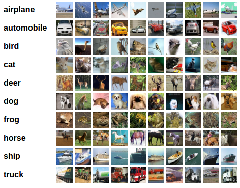
Getting a real classifier to work might help cement the workflow a bit more. CIFAR10 is a dataset of 50k tiny training images split into 10 classes.

We will do the following steps in order:

• Load CIFAR10 training and test datasets
• Define a Convolution Neural Network
• Define a loss function
• Train the network on the training data
• Test the network on the test data

Loading the Dataset

using Statistics
using Flux, Flux.Optimise
using MLDatasets: CIFAR10
using Images.ImageCore
using Flux: onehotbatch, onecold
using Base.Iterators: partition
using CUDA

This image will give us an idea of what we are dealing with.

train_x, train_y = CIFAR10.traindata(Float32)
labels = onehotbatch(train_y, 0:9)

The train_x contains 50000 images converted to 32 X 32 X 3 arrays with the third dimension being the 3 channels (R,G,B). Let's take a look at a random image from the train_x. For this, we need to permute the dimensions to 3 X 32 X 32 and use colorview to convert it back to an image.

using Plots
image(x) = colorview(RGB, permutedims(x, (3, 2, 1)))
plot(image(train_x[:,:,:,rand(1:end)]))

We can now arrange the training data in batches of say, 1000 and keep a validation set to track our progress. This process is called minibatch learning, which is a popular method of training large neural networks. Rather that sending the entire dataset at once, we break it down into smaller chunks (called minibatches) that are typically chosen at random, and train only on them. It is shown to help with escaping saddle points.

The first 49k images (in batches of 1000) will be our training set, and the rest is for validation. partition handily breaks down the set we give it in consecutive parts (1000 in this case).

train = ([(train_x[:,:,:,i], labels[:,i]) for i in partition(1:49000, 1000)]) |> gpu
valset = 49001:50000
valX = train_x[:,:,:,valset] |> gpu
valY = labels[:, valset] |> gpu

Defining the Classifier

Now we can define our Convolutional Neural Network (CNN).

A convolutional neural network is one which defines a kernel and slides it across a matrix to create an intermediate representation to extract features from. It creates higher order features as it goes into deeper layers, making it suitable for images, where the strucure of the subject is what will help us determine which class it belongs to.

m = Chain(
  Conv((5,5), 3=>16, relu),
  MaxPool((2,2)),
  Conv((5,5), 16=>8, relu),
  MaxPool((2,2)),
  x -> reshape(x, :, size(x, 4)),
  Dense(200, 120),
  Dense(120, 84),
  Dense(84, 10),
  softmax) |> gpu

We will use a crossentropy loss and an Momentum optimiser here. Crossentropy will be a good option when it comes to working with mulitple independent classes. Momentum gradually lowers the learning rate as we proceed with the training. It helps maintain a bit of adaptivity in our optimisation, preventing us from over shooting from our desired destination.

using Flux: crossentropy, Momentum

loss(x, y) = sum(crossentropy(m(x), y))
opt = Momentum(0.01)

We can start writing our train loop where we will keep track of some basic accuracy numbers about our model. We can define an accuracy function for it like so.

accuracy(x, y) = mean(onecold(m(x), 0:9) .== onecold(y, 0:9))

Training the Classifier

Training is where we do a bunch of the interesting operations we defined earlier, and see what our net is capable of. We will loop over the dataset 10 times and feed the inputs to the neural network and optimise.

epochs = 10

for epoch = 1:epochs
  for d in train
    gs = gradient(params(m)) do
      l = loss(d...)
    end
    update!(opt, params(m), gs)
  end
  @show accuracy(valX, valY)
end

Seeing our training routine unfold gives us an idea of how the network learnt the function. This is not bad for a small hand-written network, trained for a limited time.

Training on a GPU

The gpu functions you see sprinkled through this bit of the code tell Flux to move these entities to an available GPU, and subsequently train on it. No extra faffing about required! The same bit of code would work on any hardware with some small annotations like you saw here.

Testing the Network

We have trained the network for 100 passes over the training dataset. But we need to check if the network has learnt anything at all.

We will check this by predicting the class label that the neural network outputs, and checking it against the ground-truth. If the prediction is correct, we add the sample to the list of correct predictions. This will be done on a yet unseen section of data.

Okay, first step. Let us perform the exact same preprocessing on this set, as we did on our training set.

test_x, test_y = CIFAR10.testdata(Float32)
test_labels = onehotbatch(test_y, 0:9)

test = gpu.([(test_x[:,:,:,i], test_labels[:,i]) for i in partition(1:10000, 1000)])

Next, display an image from the test set.

plot(image(test_x[:,:,:,rand(1:end)]))

The outputs are energies for the 10 classes. Higher the energy for a class, the more the network thinks that the image is of the particular class. Every column corresponds to the output of one image, with the 10 floats in the column being the energies.

Let's see how the model fared.

ids = rand(1:10000, 5)
rand_test = test_x[:,:,:,ids] |> gpu
rand_truth = test_y[ids]
m(rand_test)

This looks similar to how we would expect the results to be. At this point, it's a good idea to see how our net actually performs on new data, that we have prepared.

accuracy(test[1]...)

This is much better than random chance set at 10% (since we only have 10 classes), and not bad at all for a small hand written network like ours.

Let's take a look at how the net performed on all the classes performed individually.

class_correct = zeros(10)
class_total = zeros(10)
for i in 1:10
  preds = m(test[i][1])
  lab = test[i][2]
  for j = 1:1000
    pred_class = findmax(preds[:, j])[2]
    actual_class = findmax(lab[:, j])[2]
    if pred_class == actual_class
      class_correct[pred_class] += 1
    end
    class_total[actual_class] += 1
  end
end

class_correct ./ class_total

The spread seems pretty good, with certain classes performing significantly better than the others. Why should that be?