Tutorial: Linear Regression

Flux is a pure Julia ML stack that allows you to build predictive models. Here are the steps for a typical Flux program:

• Provide training and test data
• Build a model with configurable parameters to make predictions
• Iteratively train the model by tweaking the parameters to improve predictions
• Verify your model

Under the hood, Flux uses a technique called automatic differentiation to take gradients that help improve predictions. Flux is also fully written in Julia so you can easily replace any layer of Flux with your own code to improve your understanding or satisfy special requirements.

The following page contains a step-by-step walkthrough of the linear regression algorithm in Julia using Flux! We will start by creating a simple linear regression model for dummy data and then move on to a real dataset. The first part would involve writing some parts of the model on our own, which will later be replaced by Flux.

Let us start by building a simple linear regression model. This model would be trained on the data points of the form (x₁, y₁), (x₂, y₂), ... , (xₙ, yₙ). In the real world, these xs can have multiple features, and the ys denote a label. In our example, each x has a single feature; hence, our data would have n data points, each point mapping a single feature to a single label.

Importing the required Julia packages -

julia> using Flux, Plots

Generating a dataset

The data usually comes from the real world, which we will be exploring in the last part of this tutorial, but we don't want to jump straight to the relatively harder part. Here we will generate the xs of our data points and map them to the respective ys using a simple function. Remember, here each x is equivalent to a feature, and each y is the corresponding label. Combining all the xs and ys would create the complete dataset.

julia> x = hcat(collect(Float32, -3:0.1:3)...)
1×61 Matrix{Float32}:
 -3.0  -2.9  -2.8  -2.7  -2.6  -2.5  …  2.4  2.5  2.6  2.7  2.8  2.9  3.0

The hcat call generates a Matrix with numbers ranging from -3.0 to 3.0 with a gap of 0.1 between them. Each column of this matrix holds a single x, a total of 61 xs. The next step would be to generate the corresponding labels or the ys.

julia> f(x) = @. 3x + 2;

julia> y = f(x)
1×61 Matrix{Float32}:
 -7.0  -6.7  -6.4  -6.1  -5.8  -5.5  …  9.5  9.8  10.1  10.4  10.7  11.0

The function f maps each x to a y, and as x is a Matrix, the expression broadcasts the scalar values using @. macro. Our data points are ready, but they are too perfect. In a real-world scenario, we will not have an f function to generate y values, but instead, the labels would be manually added.

julia> x = x .* reshape(rand(Float32, 61), (1, 61));

Visualizing the final data -

julia> plot(vec(x), vec(y), lw = 3, seriestype = :scatter, label = "", title = "Generated data", xlabel = "x", ylabel= "y");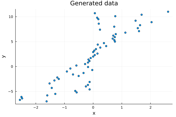

The data looks random enough now! The x and y values are still somewhat correlated; hence, the linear regression algorithm should work fine on our dataset.

We can now proceed ahead and build a model for our dataset!

Building a model

A linear regression model is defined mathematically as -

\[model(W, b, x) = Wx + b\]

where W is the weight matrix and b is the bias. For our case, the weight matrix (W) would constitute only a single element, as we have only a single feature. We can define our model in Julia using the exact same notation!

julia> custom_model(W, b, x) = @. W*x + b
custom_model (generic function with 1 method)

The @. macro allows you to perform the calculations by broadcasting the scalar quantities (for example - the bias).

The next step would be to initialize the model parameters, which are the weight and the bias. There are a lot of initialization techniques available for different machine learning models, but for the sake of this example, let's pull out the weight from a uniform distribution and initialize the bias as 0.

julia> W = rand(Float32, 1, 1)
1×1 Matrix{Float32}:
 0.99285793

julia> b = [0.0f0]
1-element Vector{Float32}:
 0.0

Time to test if our model works!

julia> custom_model(W, b, x) |> size
(1, 61)

julia> custom_model(W, b, x)[1], y[1]
(-1.6116865f0, -7.0f0)

It does! But the predictions are way off. We need to train the model to improve the predictions, but before training the model we need to define the loss function. The loss function would ideally output a quantity that we will try to minimize during the entire training process. Here we will use the mean sum squared error loss function.

julia> function custom_loss(weights, biases, features, labels)
           ŷ = custom_model(weights, biases, features)
           sum((labels .- ŷ).^2) / length(features)
       end;

julia> custom_loss(W, b, x, y)
23.772217f0

Calling the loss function on our xs and ys shows how far our predictions (ŷ) are from the real labels. More precisely, it calculates the sum of the squares of residuals and divides it by the total number of data points.

We have successfully defined our model and the loss function, but surprisingly, we haven't used Flux anywhere till now. Let's see how we can write the same code using Flux.

julia> flux_model = Dense(1 => 1)
Dense(1 => 1)       # 2 parameters

A Dense(1 => 1) layer denotes a layer of one neuron with one input (one feature) and one output. This layer is exactly same as the mathematical model defined by us above! Under the hood, Flux too calculates the output using the same expression! But, we don't have to initialize the parameters ourselves this time, instead Flux does it for us.

julia> flux_model.weight, flux_model.bias
(Float32[-1.2678515;;], Float32[0.0])

Now we can check if our model is acting right. We can pass the complete data in one go, with each x having exactly one feature (one input) -

julia> flux_model(x) |> size
(1, 61)

julia> flux_model(x)[1], y[1]
(-1.8525281f0, -7.0f0)

It is! The next step would be defining the loss function using Flux's functions -

julia> function flux_loss(flux_model, features, labels)
           ŷ = flux_model(features)
           Flux.mse(ŷ, labels)
       end;

julia> flux_loss(flux_model, x, y)
22.74856f0

Everything works as before! It almost feels like Flux provides us with smart wrappers for the functions we could have written on our own. Now, as the last step of this section, let's see how different the flux_model is from our custom_model. A good way to go about this would be to fix the parameters of both models to be the same. Let's change the parameters of our custom_model to match that of the flux_model -

julia> W = Float32[1.1412252]
1-element Vector{Float32}:
 1.1412252

To check how both the models are performing on the data, let's find out the losses using the loss and flux_loss functions -

julia> custom_loss(W, b, x, y), flux_loss(flux_model, x, y)
(22.74856f0, 22.74856f0)

The losses are identical! This means that our model and the flux_model are identical on some level, and the loss functions are completely identical! The difference in models would be that Flux's Dense layer supports many other arguments that can be used to customize the layer further. But, for this tutorial, let us stick to our simple custom_model.

Training the model

Let's train our model using the classic Gradient Descent algorithm. According to the gradient descent algorithm, the weights and biases should be iteratively updated using the following mathematical equations -

\[\begin{aligned} W &= W - \eta * \frac{dL}{dW} \\ b &= b - \eta * \frac{dL}{db} \end{aligned}\]

Here, W is the weight matrix, b is the bias vector, $\eta$ is the learning rate, $\frac{dL}{dW}$ is the derivative of the loss function with respect to the weight, and $\frac{dL}{db}$ is the derivative of the loss function with respect to the bias.

The derivatives are calculated using an Automatic Differentiation tool, and Flux uses Zygote.jl for the same. Since Zygote.jl is an independent Julia package, it can be used outside of Flux as well! Refer to the documentation of Zygote.jl for more information on the same.

Our first step would be to obtain the gradient of the loss function with respect to the weights and the biases. Flux re-exports Zygote's gradient function; hence, we don't need to import Zygote explicitly to use the functionality.

julia> dLdW, dLdb, _, _ = gradient(custom_loss, W, b, x, y);

We can now update the parameters, following the gradient descent algorithm -

julia> W .= W .- 0.1 .* dLdW
1-element Vector{Float32}:
 1.8144473

julia> b .= b .- 0.1 .* dLdb
1-element Vector{Float32}:
 0.41325632

The parameters have been updated! We can now check the value of the loss function -

julia> custom_loss(W, b, x, y)
17.157953f0

The loss went down! This means that we successfully trained our model for one epoch. We can plug the training code written above into a loop and train the model for a higher number of epochs. It can be customized either to have a fixed number of epochs or to stop when certain conditions are met, for example, change in loss < 0.1. The loop can be tailored to suit the user's needs, and the conditions can be specified in plain Julia!

Let's plug our super training logic inside a function and test it again -

julia> function train_custom_model!(f_loss, weights, biases, features, labels)
           dLdW, dLdb, _, _ = gradient(f_loss, weights, biases, features, labels)
           @. weights = weights - 0.1 * dLdW
           @. biases = biases - 0.1 * dLdb
       end;

julia> train_custom_model!(custom_loss, W, b, x, y);

julia> W, b, custom_loss(W, b, x, y)
(Float32[2.340657], Float32[0.7516814], 13.64972f0)

It works, and the loss went down again! This was the second epoch of our training procedure. Let's plug this in a for loop and train the model for 30 epochs.

julia> for i = 1:40
          train_custom_model!(custom_loss, W, b, x, y)
       end

julia> W, b, custom_loss(W, b, x, y)
(Float32[4.2422233], Float32[2.2460847], 7.6680417f0)

There was a significant reduction in loss, and the parameters were updated!

We can train the model even more or tweak the hyperparameters to achieve the desired result faster, but let's stop here. We trained our model for 42 epochs, and loss went down from 22.74856 to 7.6680417f. Time for some visualization!

Results

The main objective of this tutorial was to fit a line to our dataset using the linear regression algorithm. The training procedure went well, and the loss went down significantly! Let's see what the fitted line looks like. Remember, Wx + b is nothing more than a line's equation, with slope = W[1] and y-intercept = b[1] (indexing at 1 as W and b are iterable).

Plotting the line and the data points using Plot.jl -

julia> plot(reshape(x, (61, 1)), reshape(y, (61, 1)), lw = 3, seriestype = :scatter, label = "", title = "Simple Linear Regression", xlabel = "x", ylabel= "y");

julia> plot!((x) -> b[1] + W[1] * x, -3, 3, label="Custom model", lw=2);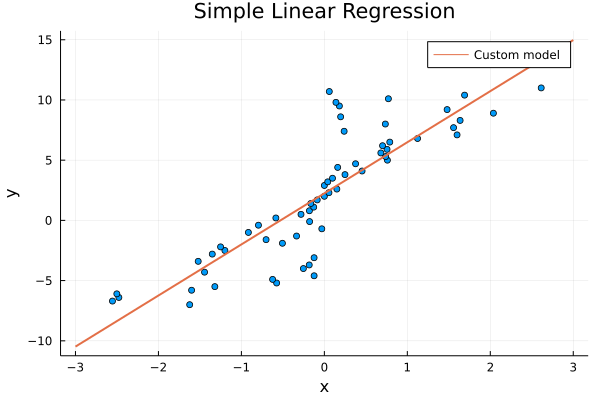

The line fits well! There is room for improvement, but we leave that up to you! You can play with the optimisers, the number of epochs, learning rate, etc. to improve the fitting and reduce the loss!

Linear regression model on a real dataset

We now move on to a relatively complex linear regression model. Here we will use a real dataset from MLDatasets.jl, which will not confine our data points to have only one feature. Let's start by importing the required packages -

julia> using Flux, Statistics, MLDatasets, DataFrames

Gathering real data

Let's start by initializing our dataset. We will be using the BostonHousing dataset consisting of 506 data points. Each of these data points has 13 features and a corresponding label, the house's price. The xs are still mapped to a single y, but now, a single x data point has 13 features.

julia> dataset = BostonHousing();

julia> x, y = BostonHousing(as_df=false)[:];

julia> x, y = Float32.(x), Float32.(y);

We can now split the obtained data into training and testing data -

julia> x_train, x_test, y_train, y_test = x[:, 1:400], x[:, 401:end], y[:, 1:400], y[:, 401:end];

julia> x_train |> size, x_test |> size, y_train |> size, y_test |> size
((13, 400), (13, 106), (1, 400), (1, 106))

This data contains a diverse number of features, which means that the features have different scales. A wise option here would be to normalise the data, making the training process more efficient and fast. Let's check the standard deviation of the training data before normalising it.

julia> std(x_train)
134.06786f0

The data is indeed not normalised. We can use the Flux.normalise function to normalise the training data.

julia> x_train_n = Flux.normalise(x_train);

julia> std(x_train_n)
1.0000844f0

The standard deviation is now close to one! Our data is ready!

Building a Flux model

We can now directly use Flux and let it do all the work internally! Let's define a model that takes in 13 inputs (13 features) and gives us a single output (the label). We will then pass our entire data through this model in one go, and Flux will handle everything for us! Remember, we could have declared a model in plain Julia as well. The model will have 14 parameters: 13 weights and 1 bias.

julia> model = Dense(13 => 1)
Dense(13 => 1)      # 14 parameters

Same as before, our next step would be to define a loss function to quantify our accuracy somehow. The lower the loss, the better the model!

julia> function loss(model, features, labels)
           ŷ = model(features)
           Flux.mse(ŷ, labels)
       end;

julia> loss(model, x_train_n, y_train)
676.1656f0

We can now proceed to the training phase!

Training the Flux model

The training procedure would make use of the same mathematics, but now we can pass in the model inside the gradient call and let Flux and Zygote handle the derivatives!

julia> function train_model!(f_loss, model, features, labels)
           dLdm, _, _ = gradient(f_loss, model, features, labels)
           @. model.weight = model.weight - 0.000001 * dLdm.weight
           @. model.bias = model.bias - 0.000001 * dLdm.bias
       end;

Contrary to our last training procedure, let's say that this time we don't want to hardcode the number of epochs. We want the training procedure to stop when the loss converges, that is, when change in loss < δ. The quantity δ can be altered according to a user's need, but let's fix it to 10⁻³ for this tutorial.

We can write such custom training loops effortlessly using Flux and plain Julia!

julia> loss_init = Inf;

julia> while true
           train_model!(loss, model, x_train_n, y_train)
           if loss_init == Inf
               loss_init = loss(model, x_train_n, y_train)
               continue
           end
           if abs(loss_init - loss(model, x_train_n, y_train)) < 1e-4
               break
           else
               loss_init = loss(model, x_train_n, y_train)
           end
       end;

The code starts by initializing an initial value for the loss, infinity. Next, it runs an infinite loop that breaks if change in loss < 10⁻³, or the code changes the value of loss_init to the current loss and moves on to the next iteration.

This custom loop works! This shows how easily a user can write down any custom training routine using Flux and Julia!

Let's have a look at the loss -

julia> loss(model, x_train_n, y_train)
27.1272f0

The loss went down significantly! It can be minimized further by choosing an even smaller δ.

Testing the Flux model

The last step of this tutorial would be to test our model using the testing data. We will first normalise the testing data and then calculate the corresponding loss.

julia> x_test_n = Flux.normalise(x_test);

julia> loss(model, x_test_n, y_test)
66.91015f0

The loss is not as small as the loss of the training data, but it looks good! This also shows that our model is not overfitting!

Summarising this tutorial, we started by generating a random yet correlated dataset for our custom model. We then saw how a simple linear regression model could be built with and without Flux, and how they were almost identical.

Next, we trained the model by manually writing down the Gradient Descent algorithm and optimising the loss. We also saw how Flux provides various wrapper functionalities and keeps the API extremely intuitive and simple for the users.

After getting familiar with the basics of Flux and Julia, we moved ahead to build a machine learning model for a real dataset. We repeated the exact same steps, but this time with a lot more features and data points, and by harnessing Flux's full capabilities. In the end, we developed a training loop that was smarter than the hardcoded one and ran the model on our normalised dataset to conclude the tutorial.